8 Chapter 4 Lab

8.1 Moving Average model (MA)

\[ X_t = \mu + Noise_t + \lambda \cdot(Noise_{t-1})\] Regression on today’s data using yesterday’s noise.

# Generate MA model with slope 0.5
x <- arima.sim(model = list(ma = 0.5), n = 100)

# Generate MA model with slope 0.9
y <- arima.sim(model = list(ma = 0.9), n = 100)

# Generate MA model with slope -0.5
z <- arima.sim(model = list(ma = -0.5), n = 100)

# Plot all three models together
plot.ts(cbind(x, y, z))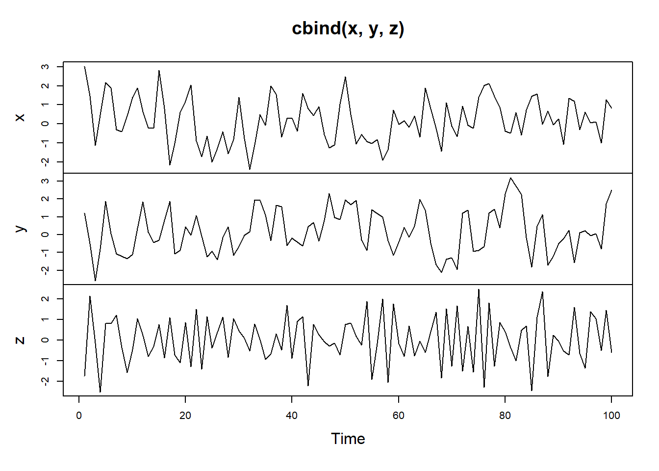

par(mfrow = c(3, 1))

# Calculate the ACF 
acf(x)
acf(y)
acf(z)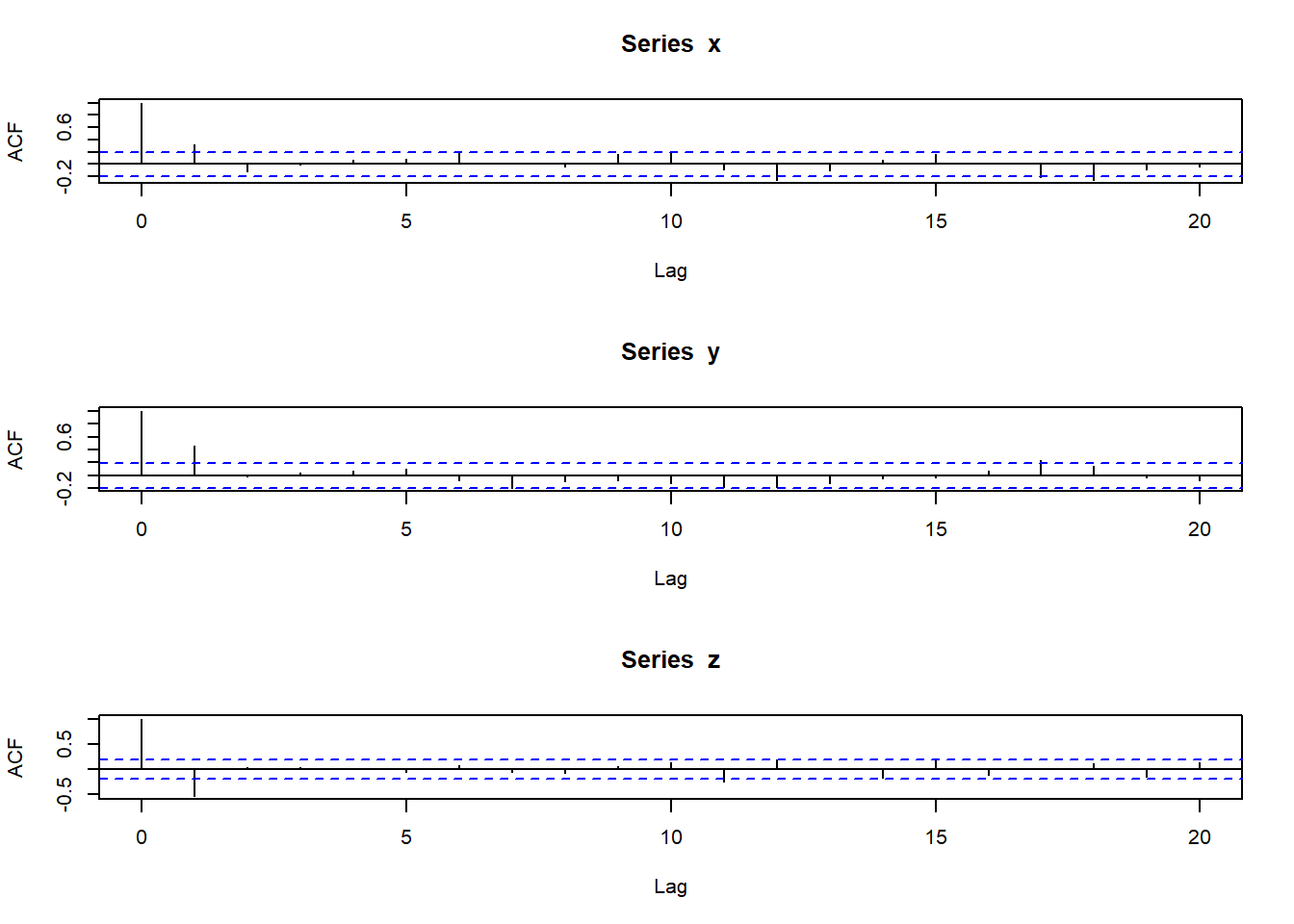

The ACF plots tell that it is appropriate to use MA(1) model to fit this data. This is expected since we used MA(1) model with different values of \(\lambda\) to simulate the data

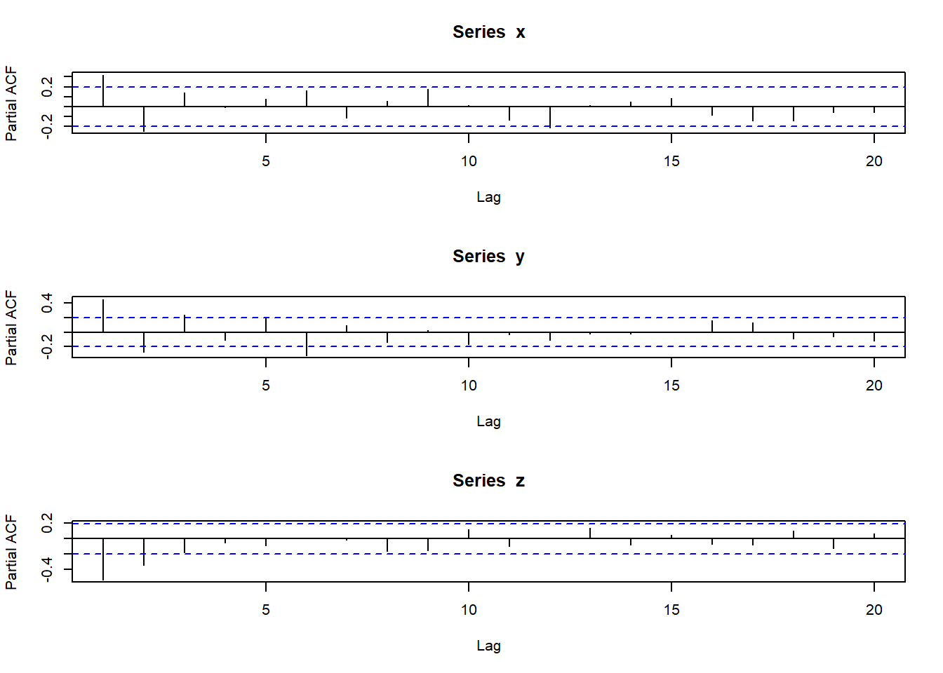
par(mfrow = c(3, 1))
pacf(x)
pacf(y)
pacf(z)